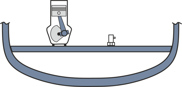
Elastic mounts are an appropriate measure to reduce the transmission of vibrations from machines to a supporting structure. We take the setup described in Figure 1 (from the previous example Bearing Structure) as example and place elastic mounts between the engine and the supporting structure. As discussed in the example Bearing Structure, it is important to consider the overall coupled system dynamics of the engine, the elastic mounting and the supporting structure. First this example will discuss the effect of elastic mounting when the engine is mounted on a structure with high impedance, e.g. a heavy concrete slap foundation. Then the model is extended to consider the dynamic characteristics of the supporting structure, e.g. the ship segment from the example Bearing Structure.
Passive isolation by elastic mounts:
In the case of a rigid mounting the vibrations of the engine and the supporting structure are the same, i.e. for the case of the rigid mounting in Figure 2 (from example Bearing Structure) the deflection of the machine xm and the deflection of the beam are identical. Putting an elastic mount between the engine and the supporting structure causes introduces a shift of phase and amplitude between the two vibration signals. Considering first a machine supported on a structure with high impedance we can observe the general effects of an elastic isolation. The transmissibility of an elastic the simple 1DOF mechanical system shown in Figure 7 can be calculated with T(s=iω)=x2/x1 =(1+[2ξs/ωi])/(1+[2ξs/ωi]+s²/[ω1]^2 ) [4].For the effective isolation the right choice of the stiffness ki and damping di is essential (see Figure 7). Independent of its internal damping, the elastic isolation is effective for frequencies above the isolation frequenciy at √2 ωi.
However, around the resonance frequency of the 1DOF system and frequencies well above the isolation frequency, the internal damping of the elastic mount has a significant effect on the vibration isolation.
In Figure 7 the transmissibility of a 1DOF system is shown for different damping ratios ξ=d_i/(2ω_i m). For ξ=0 a damping free case is considered. In this case around the resonance frequency of the 1DOF system the amplitude of the transmissibility goes to infinity (this means the vibration is not reduced but actually amplified). Above the isolation frequency the isolation increase by 40 dB/decade. Increasing the internal damping of the elastic mount the amplification around the resonance frequency of the 1DOF system is reduced. However, as a trade-off also the isolation effect in the frequecy region above the isolation frequency is reduced.
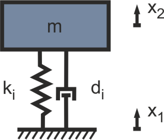 | 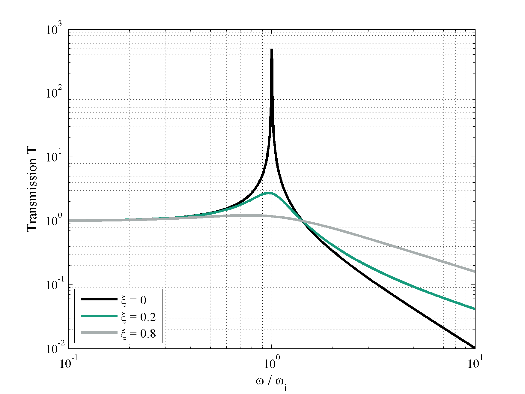 |
Figure 7: a) Mechanical setup of an isolator and b) calculated transmission | |
In Figure 7 the transmission of the isolation regarding different damping factores ξ=d_i/(2ω_i m). For ξ=0 a damping free case is considered, where the amplitude goes to infinity for the resonance frequency. Above the isolation frequency an increase of the isolation of 40 dB/decade can be seen. For an increase of the damping the resonance is reduced, but also the isolation effect is reduced.
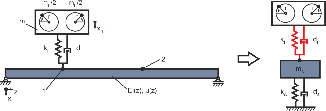
Figure 8: Simplification of the structure with an elastic mounting of the excitation
The stiffness ki of the isolation has to be designed with respect to the mass of the machine m. Here it is important, that the operating speed nu=30ωu/π is in the domain of the isolation. By this means the requirement ωu>ωi has to be fulfilled. The isolation frequency can be calculated with respect to the natural frequency of the oscillator, set up by the stiffness ki and the mass m under the assumption, that ki < k1 (stiffness of the structure at the installation site) to ωi^2≈(2k_i)/m [1]. Assuming the lowest operating speed for the regarded example is 1200 rpm with a mass of the machine m = 8000 kg the stiffness has to be ki < 2.1e6 N/m (in this example a value of ki = 2e6 N/m). By this means the isolation frequency can be calculated to fi=√(k_i/m)/(2π)=9.2 Hz. The damping of the isolation di is important for the limitation of the amplitude of the natural frequency of the setup while passing through in the run-up of the machine. On the other hand one has to be careful to choose the right damping in terms with respect to the efficiency of the isolation effect. Here a damping of di = 1000 kg*s is used.
Implementation in Simulink®:
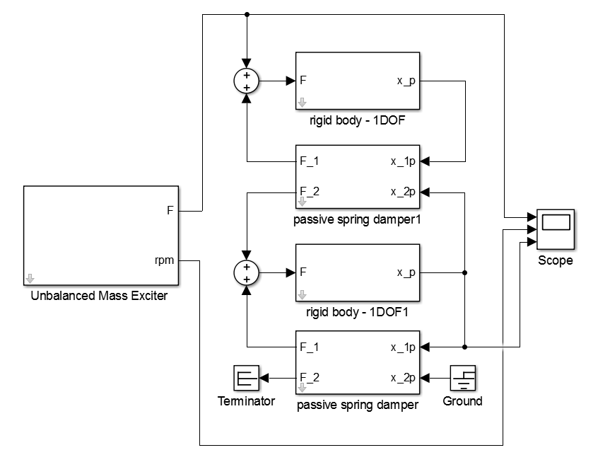
Figure 9: Simulink® block-diagram of the damped harmonic oscillator with an isolation of the excitation
For time-domain simulations a Simulink® model is implemented as seen in Figure 9. For the parametrization the properties listed in Table 1 are used.
Results:
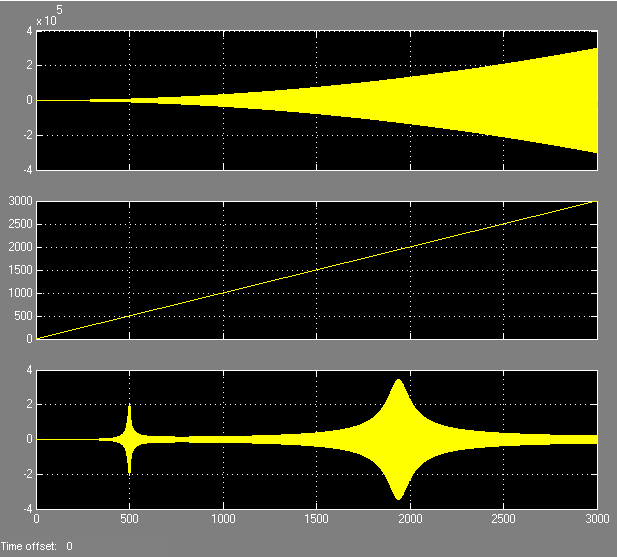
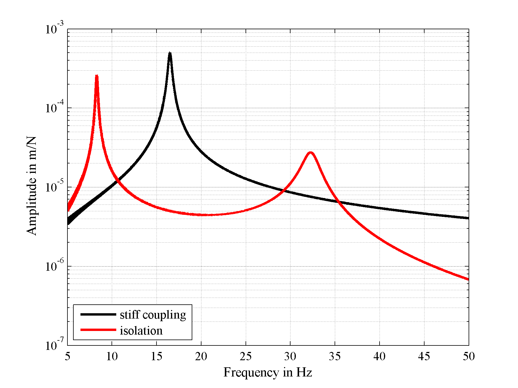
In Figure 10 the results in the time and frequency-domain can be seen. The frequency domain is evaluated by the use of the ma_frequency_response function:
[FREQ,AMPL,PHAS]=ma_frequency_response(ScopeData.time, ScopeData.signals(1).values,
ScopeData.signals(3).values,{0,50});
[FREQ_Isolation,AMPL_Isolation,PHAS_Isolation]=ma_frequency_response(ScopeData_Isolation.time, ScopeData_Isolation.signals(1).values, ScopeData_Isolation.signals(3).values,{0,50});
figure
semilogy(FREQ,AMPL,’k’,’LineWidth’,2); hold on;
semilogy(FREQ_Isolation,AMPL_Isolation,’r’,’LineWidth’,2);
hold off;
grid on
xlabel(‘Frequency in Hz’)
ylabel(‘Amplitude in m/N’)
legend(‘stiff coupling’,’isolation’,’Location’,’SouthWest’)
xlim([5 50])
Clearly the main resonance at 16.5 Hz is reduced. An additional resonance occurs at 8.3 Hz, but below the operational domain. The main resonance shifts to 32.3 Hz, what is still in the operational domain, but with much lower amplitude.
 |  |
For an analytical comparison the system matrices can be derived using the function ma_MOSys from the structure and vibration toolbox:
% jData definition of sys1
jData = [1 282.6; 2 600];
% kData definition of sys1
kData = [1 inf 9470328 2000;
1 2 2e6 1000];
% Sys1 = ma_MOSys(jData,kData)
% originF definition
originFvalue = 2;
% outputP definition
outputPvalue = 1;
Sys1 = ma_MOSys(jData,kData,’originF’,originFvalue,’outputP’,outputPvalue);
By this means the system is transferred to a state-space system and the eigenvalues are calculated:
ss = ma_MOSysGetSS(Sys1);
eig(ss)
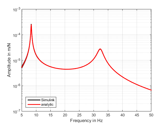
As result the eigenfrequencies 32.3 Hz and 8.29 Hz are calculated which match the Simulink® simulation. For a match of the amplitudes the frequency response functions are compared:
freq_analytic=1:0.1:50;
[mag_analytic, phase_analytic]=bode(ss,freq*2*pi);
mag_analytic=reshape(mag_analytic,1,length(freq));
[FREQ_Isolation,AMPL_Isolation,PHAS_Isolation]=ma_frequency_response(ScopeData_Isolation.time, ScopeData_Isolation.signals(1).values, ScopeData_Isolation.signals(3).values,{0,50});
figure
semilogy(FREQ_Isolation,AMPL_Isolation,’k’,’LineWidth’,2); hold on;
semilogy(freq_analytic,mag_analytic,’r’,’LineWidth’,2);
hold off;
grid on
xlabel(‘Frequency in Hz’)
ylabel(‘Amplitude in m/N’)
legend(‘Simulink’,’analytic’,’Location’,’SouthWest’)
xlim([5 50])