Passive measures for vibration minimisation using the example of a load-bearing structure with supported machine :: Tutorial (Fraunhofer LBF) |
Problem description
Unwanted vibrations often occur during the operation of machines. These vibrations can impair the function of the machine and, in the worst case, lead to premature material failure. In addition, the resulting vibrations and the associated noise generation are harmful to the environment. Particularly in the case of resonance, when the excitation frequency coincides with the natural frequency of the system, this leads to an amplification of the resulting vibration amplitudes. It is therefore an important task of machine dynamics to reduce such undesirable vibrations through suitable design measures. The resulting vibrations are not limited to individual components; neighbouring structures are also stimulated to vibrate by the interaction of forces and movements. Therefore, not only the dynamic behaviour of the machine itself must be considered, but also the properties of the installation site – in particular the bearing points – have a major influence on the vibration behaviour of the overall system.
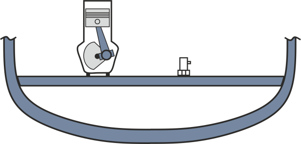
The ma_Toolbox provides content with which the dynamic behaviour can be modelled and the influence of design measures on this behaviour can be investigated. The procedure is shown below using the example of an internal combustion engine in a ship’s hull (see figure 1). For this purpose, the real system is transferred to a suitable model and the dynamic behaviour of the overall system is simulated. The engine is first considered to be fixed to the elastic structure of the mounting location and the influence of the engine-induced vibrations on this model is determined. Subsequently, possible passive methods for vibration reduction (vibration isolation by optimising the bearing points, vibration damping by means of a suitable additional mass) are investigated and the mechanical system is extended by appropriate components.
Mechanical substitute system
Real structures often have a high degree of complexity. For this reason, it makes sense to perform basic analyses on simplified structures. For this purpose, the real system is transformed into a mechanical substitute system. This must reproduce the properties of the real system to be analysed with sufficient accuracy. The engine is assumed to be a 12-cylinder engine with a total weight of 600 kg. Each cylinder has a mass of 16 kg with a stroke of 190 mm. The typical frequency range is 13 – 34 Hz, which corresponds to a speed of 800 – 2000 rpm.
The idealised motor can be represented as an unbalance exciter with the total mass mm, the rotational frequency Ω and the unbalance mass mu, which moves around the radius r. The resulting force of the unbalance exciter is given by 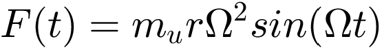 . In the simplest case, the ship’s floor is modelled as an elastic beam with the modulus of elasticity E, the area moment of inertia I and the length-related mass μ. This beam can be converted into an equivalent spring-mass-damper system with one degree of freedom. For this, the vibration properties of the beam are first calculated and then the parameters of the spring-mass damper system (ms, ks and ds) are determined so that they reflect the vibration behaviour of the system at a specific position. In the following, it is assumed for the sake of simplicity that the motor is located in the centre of the beam (position 1, z = L/2) and that this position corresponds to the position at which the movement of the structure
 ![]() is measured (position 2) (see figure 2). [1]
is measured (position 2) (see figure 2). [1]
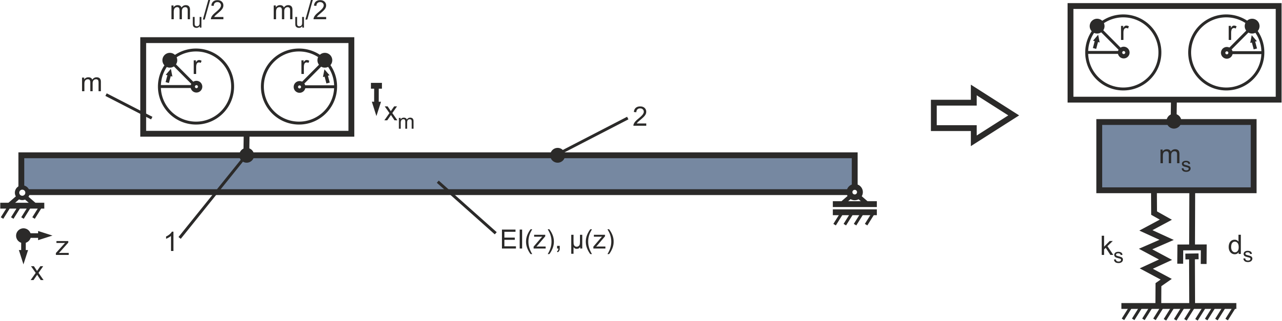
Figure 2: Mechanical equivalent system of the structure as an elastically supported beam and equivalent mass-spring-damper system with one degree of freedom
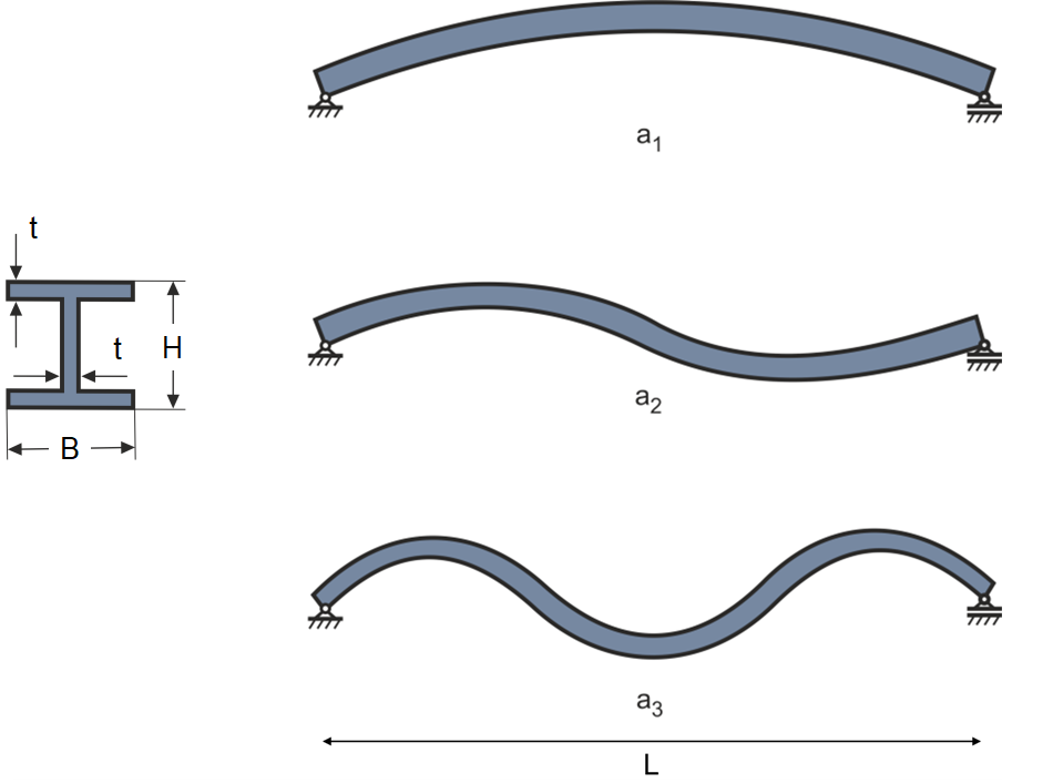
Vibration characteristics of the beam: An I-section with the dimensions H = 0.2 m, B = 0.2 m, t = 0.02 m and a length L = 4.8 m is selected for the geometry of the beam (figure 3). The material is assumed to be steel with a modulus of elasticity of E = 2.1e+11 N/m2 and a density of ρ = 7850 kg/m3. With these values, the moment of inertia can be calculated with  = 7.1893e-05 m4 and the cross-sectional area with
 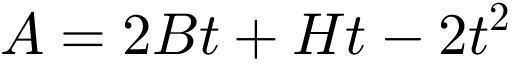 = 0.0112 m2. [2] With the length-related mass μ = ρA = 87.92 kg/m and assuming negligibly low damping, the first three natural frequencies result from
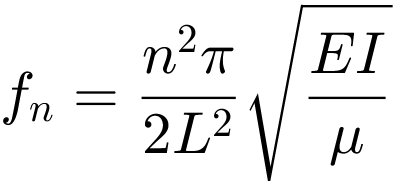
with n = 1, 2, 3 to f1 = 28.252 Hz, f2 = 113.01 Hz and f3 = 254.27 Hz. Figure 3 shows the corresponding eigenmodes a1, a2 and a3. The first resonant frequency of the basic structure is of particular interest in the following, as it lies within the frequency range of the motor.
In order to obtain an equivalent single-mass oscillator, an equivalent mass and an equivalent stiffness are calculated, taking into account the bending shape and the potential and kinetic energy. The equivalent mass
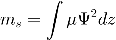
results for the sinusoidal eigenmode shown in Figure 3 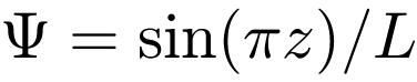 at the location
  to
to 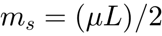 = 211.01 kg. Taking into account the concentrated total mass of the motor mm, the equivalent total mass is
  = 811.01 kg. The equivalent stiffness is
 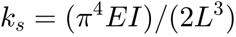 = 6.649e+06 N/m. A hysteretic damping of approximately η = 4% is assumed as the damping of the structure. The equivalent modal damping thus results in
 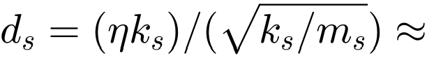 1000 kg/s. [3]
Implementation in Simulink
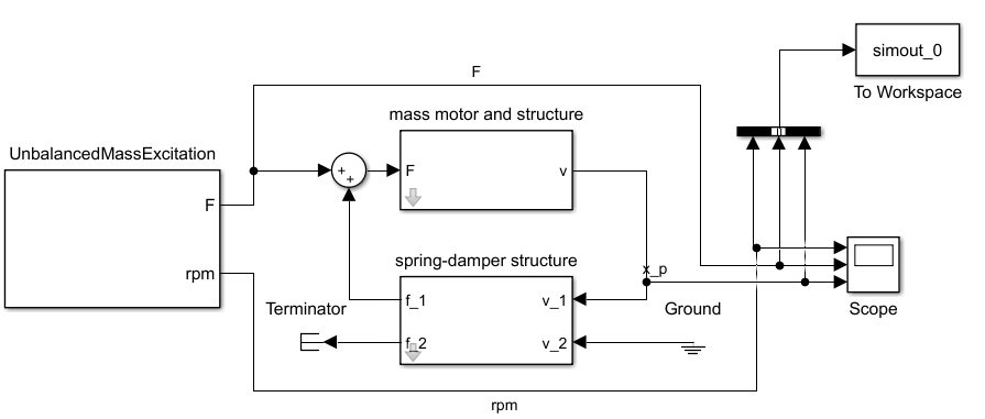
Figure 4: Simulink model of the damped single-mass oscillator
The time domain simulations are carried out with Simulink. For this purpose, the model shown in Figure 4 is created, whereby the simulations are performed with the fixed-step solver and a fixed sampling rate of ts = 0.001 s for a time from 0 to t_end = 30 s. To implement the model, the blocks Stiffness1DOF, RigidBody1DOF and UnbalancedMassExcitation from the “Structure and Vibration” toolbox are used and parameterised with the previously determined values. A speed range of 0 to 3000 rpm is selected for the unbalance exciter with an acceleration rate of 100 1/min/s. The parameters of the blocks are summarised in Table 1:
Table 1. Parameterisation of the model
| BlockName | BlockType | BlockProperty | VariableName | PropertValue |
|---|---|---|---|---|
| Mass motor and structure | RigidBody1DOF | inertia (weight of the mass [kg] or moment of inertia [kgm^2]) | m_ges | 811.01 |
| Spring-damper strukture | Stiffness1DOF | stiffness [N/m] | k_s | 6.649e+06 |
| damping coefficient [Ns/m] | d_s | 1000 | ||
| UnbalancedMassExcitation | UnbalancedMassExcitation | unbalanced mass [kg] | m_u | 16 |
| eccentricity of the unbalance [m] | r_u | 0.19 | ||
| idle speed [1/min] | rpm0 | 0 | ||
| speed ratio at start-up [1/min/s] | rpm_ratio | 100 | ||
| sample time [s] | ts | 0.001 |
For further processing of the data outside of Simulink, the signals are exported as “Structure with Time” (simout_0) using the Simulink To Workspace block. Figure 5 shows the results of the simulation in the time domain. The top two axes show the speed of the motor and the force resulting from the unbalance. The lower axis shows the speed of the beam at position 1. It is clearly recognisable that this increases sharply after about 9 seconds. This is due to the direct coupling of the machine mass and the beam.
▾ Show source code
% Display simulation data in time domain
time_0 = simout_0.time;
rpm_0  = simout_0.signals.values(:,1);
F_0    = simout_0.signals.values(:,2);
x_0    = simout_0.signals.values(:,3);

h = figure();
subplot(3,1,1);
title('Simulation result - Time domain')
ma_graphics.plot(time_0,rpm_0);
ylabel('rpm');

subplot(3,1,2);
ma_graphics.plot(time_0,F_0);
ylabel('F');

subplot(3,1,3);
ma_graphics.plot(time_0,x_0);
ylabel('$\dot{x}$','Interpreter','latex','FontSize',15);
xlabel('time');
ylim([-13,13]);
ah = findobj(h,'type','axes');
set(ah,'XGrid','on','YGrid','on');
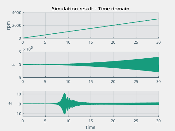
Figure 5: Simulation results in the time domain
In order to analyse the results more precisely, the simulation results are transformed into the frequency range using the function ma_frequency_response.
▾ Show source code
% Display simulation results in frequency domain
ma_frequency_response(time_0, F_0, x_0,{0,50});
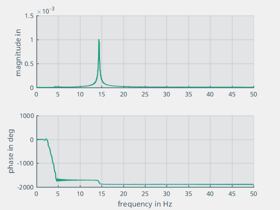
Figure 6: Simulation results in the frequency range
The resonance at a frequency of approx. 14 Hz is clearly recognisable. The observed resonance corresponds to the result of the analytically calculated natural frequency of the system 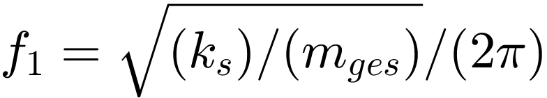 = 14.411 Hz.
Passive isolation using elastic bearings
By using elastic bearings, the dynamic forces that are introduced into a structure by a machine can be reduced. In the following, the procedure is shown using the marine engine considered in this tutorial. In addition to the dynamic behaviour of the machine, the properties of the basic structure, in this case the ship, must also be taken into account. In the case of a rigid mounting, as considered in the previous section, the displacements of the structure xs and the motor xm are identical. Vibration isolation can be achieved with an additional spring-damper element (ki, di). A suitable choice of stiffness and damping parameters is crucial for this. To describe the isolation effect, the system consisting of motor mass and isolator-spring-damper is initially idealised (see figure 7).
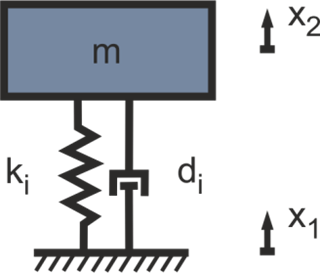
Figure 7: Mechanical structure of an insulator
The transmission behaviour of the isolator shown in Figure 7 is represented by the function

where  and
and  . The isolation effect occurs above the effective frequency
  . Figure 8 shows the transmission behaviour of the isolator as a function of the damping factor ξ. In the undamped case (ξ = 0), the amplitude at resonance approaches infinity. Above the isolation frequency, the transmission decreases with a value of 40 dB/decade. By increasing the damping, the amplitude at the point of resonance is reduced, but at the same time the isolation effect is reduced. [4]

Figure 8: Transmission of the isolator
In order to model vibration isolation by means of an elastic bearing of the motor, the model shown in Figure 2 is extended by a spring-damper element (see Figure 9). The stiffness of the isolation ki must be selected taking into account the machine mass mm = 600 kg. It is important to select ki in such a way that the isolation effect covers the operating speed range  . In this specific case, this means that the insulation frequency ωi must be selected so that the effective isolation effect (
![]() ) starts below the lower speed limit of 800 rpm or a circular frequency of ω = 83.776 Hz. Assuming that ki < ks, the required insulation frequency can be determined with
) starts below the lower speed limit of 800 rpm or a circular frequency of ω = 83.776 Hz. Assuming that ki < ks, the required insulation frequency can be determined with 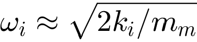 . This means that the stiffness must be less than 2.1055e+06 N/m. In this example, a value of 2000000 N/m is selected. This configuration results in an isolation frequency of
 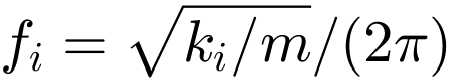 = 9.1888 Hz.
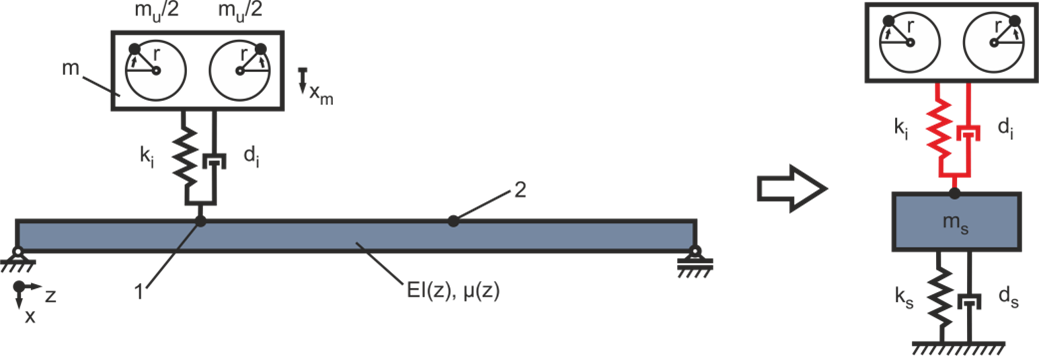
Figure 9: Mechanical model with an elastic support of the excitation
The damping of the isolation di is important in order to limit the amplitude of the resonance frequency, as the excitation passes through it during run-up. On the other hand, it is important not to set the damping too high with regard to the isolation effect. In the following, a damping factor ζ of approx. 2% is assumed. This results in the damping constant of the isolator di with 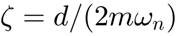 . In this example, an damping constant di = 1400 kg*s is assumed.
Implementation in Simulink
Figure 10 shows the Simulink model extended by the elastic support. The model parameters are listed in Table 2.
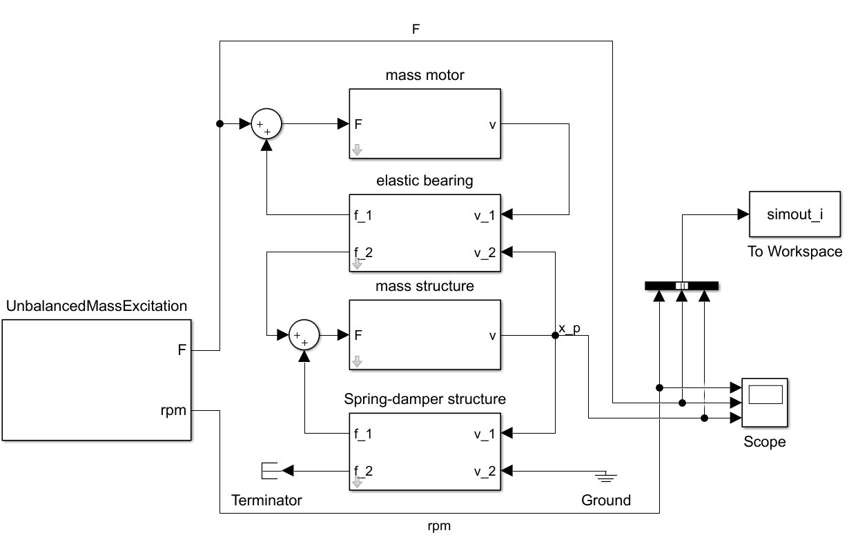
Figure 10: Simulink model of the elastically mounted motor
Table 2. Parameterisation of the model
| BlockName | BlockType | BlockProperty | VariableName | PropertValue |
|---|---|---|---|---|
| Mass motor | RigidBody1DOF | inertia (weight of the mass [kg] or moment of inertia [kgm^2]) | m_m | 600 |
| Mass structure | RigidBody1DOF | inertia (weight of the mass [kg] or moment of inertia [kgm^2]) | m_s | 211.01 |
| Spring-damper structure | Stiffness1DOF | stiffness [N/m] | k_s | 6.649e+06 |
| damping coefficient [Ns/m] | d_s | 1000 | ||
| Elastic bearing | Stiffness1DOF | stiffness [N/m] | k_i | 2000000 |
| damping coefficient [Ns/m] | d_i | 1400 | ||
| UnbalancedMassExcitation | UnbalancedMassExcitation | unbalanced mass [kg] | m_u | 16 |
| eccentricity of the unbalance [m] | r_u | 0.19 | ||
| idle speed [1/min] | rpm0 | 0 | ||
| speed ratio at start-up [1/min/s] | rpm_ratio | 100 | ||
| sample time [s] | ts | 0.001 |
The simulation results simout_i are further processed in Matlab. Figure 11 shows the results of the simulation in the time domain.
▾ Show source code
% Display simulation data in time domain

time_i = simout_i.time;
rpm_i  = simout_i.signals.values(:,1);
F_i    = simout_i.signals.values(:,2);
x_i    = simout_i.signals.values(:,3);

h = figure();
subplot(3,1,1);
title('Simulation result - Time domain')
ma_graphics.plot(time_i,rpm_i);
ylabel('rpm');

subplot(3,1,2);
ma_graphics.plot(time_i,F_i);
ylabel('F');

subplot(3,1,3);
ma_graphics.plot(time_i,x_i);
ylabel('$\dot{x}$','Interpreter','latex','FontSize',15);
xlabel('time');
ylim([-6,6]);
ah = findobj(h,'type','axes');
set(ah,'XGrid','on','YGrid','on');

Figure 11: Simulation results in the time domain
In the following, the results in the frequency range are considered and the simulation results of the elastically mounted motor are compared with those of the rigidly connected motor (Figure 12). The elastic bearing shifted the first resonance frequency to 32 Hz. It is still inside the operating range but with a significantly lower amplitude. At 8 Hz an additional resonance occurs, which is outside the operating range of the excitation.
▾ Show source code
% Display simulation results in frequency domain

[FREQ_0,AMPL_0,PHAS_0] = ma_frequency_response(time_0, F_0, x_0,{0,50},'window',true);
[FREQ_i,AMPL_i,PHAS_i] = ma_frequency_response(time_i, F_i, x_i,{0,50},'window',true);

figure();
ma_graphics.semilogy(FREQ_0,AMPL_0);
hold on;
ma_graphics.semilogy(FREQ_i,AMPL_i);
grid on
xlabel('Frequency in Hz')
ylabel('Amplitude in m/N')
legend('Stiff coupling','Isolation','Location','SouthWest')
xlim([5 50])

% display operation range
fu_min = 13;
fu_max = 33;

rectangle('Position',[fu_min,1e-6,fu_max-fu_min,1.9e-4],'FaceColor',[0 .5 .5 0.2],'EdgeColor','b', 'LineWidth',1);
% push rectangle (last plot) to the back
h = get(gca,'Children');
set(gca,'Children',[h(2:end)',h(1)]);
text(14,1.5e-6,'Operation range')
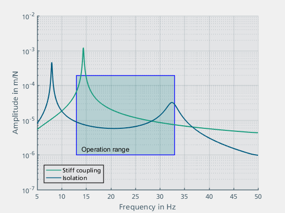
Figure 12: Results in the frequency range
The next section examines the extent to which the resonances that occur can be reduced by using a vibration damper. First, however, the class ma_mosys of the ma_Toolbox is used to analytically analyse the simulation results.
Analytical solution using the ma_mosys class
The class can be used to set up multi-mass oscillators and analyse the oscillation properties of the system. To do so, an object of the class is first created with the corresponding system matrices (jData, kData). The system is then transferred to the state space (state space model) and the eigenvalues are calculated.
▾ Show source code
% Define the mass matrix of the system, where the first entry defines the mass annotation
jData = [1 m_s;
         2 m_m];

% Define arrangement of the masses and the spring and damper values of the respective connections
kData = [1 inf k_s d_s;
         1 2   k_i d_i];

% Force application points of the system
originFvalue = 2;

% Output velocity masses of the system
outputPvalue = 1;

system = ma_mosys(jData,kData,'originF',originFvalue,'outputP',outputPvalue);

% Create the state-space model
system.getSS;

% Use the matlab built-in function eig to calculate the eigen values
eigenValues = eig(system.SS);
eigenFrq_i = unique(abs(eigenValues))/(2*pi);
The analytically calculated frequencies 7.9778 Hz and 32.541 Hz correspond to the results from Simulink. For a comparison of the amplitude response, the transfer functions are compared in Figure 13:
▾ Show source code
freq_analytic=0:0.1:50;
[mag_analytic, phase_analytic]=bode(system.SS,freq_analytic*2*pi);
mag_analytic = reshape(mag_analytic,1,length(freq_analytic));

h = figure();
ma_graphics.semilogy(FREQ_i,AMPL_i);
hold on;
ma_graphics.semilogy(freq_analytic,mag_analytic);
hold off;
grid on
xlabel('Frequency in Hz')
ylabel('Amplitude in m/N')
legend('Simulink','Analytic','Location','SouthWest')
xlim([5 50])
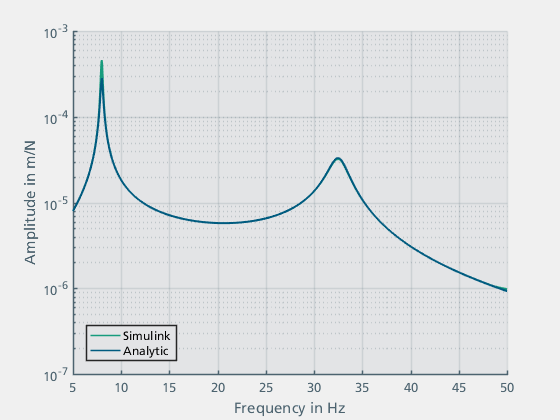
Figure 13: Comparison of the Simulink model with the analytical solution
It can be clearly seen that the results from the simulation in Simulink and the solution of the analytical model match.
Vibration reduction with a vibration absorber
It is possible to reduce vibrations in a structure through additional structural dynamic measures, such as a vibration absorber. This reduces the amplitude of a structural resonance. The procedure is first illustrated using the rigidly mounted motor. For this purpose, the equivalent system shown in Figure 2 is extended by a corresponding absorber (see Figure 14). In the equivalent spring-damper system, the motor mass and the absorber are assumed to be superimposed in the position z = L/2.
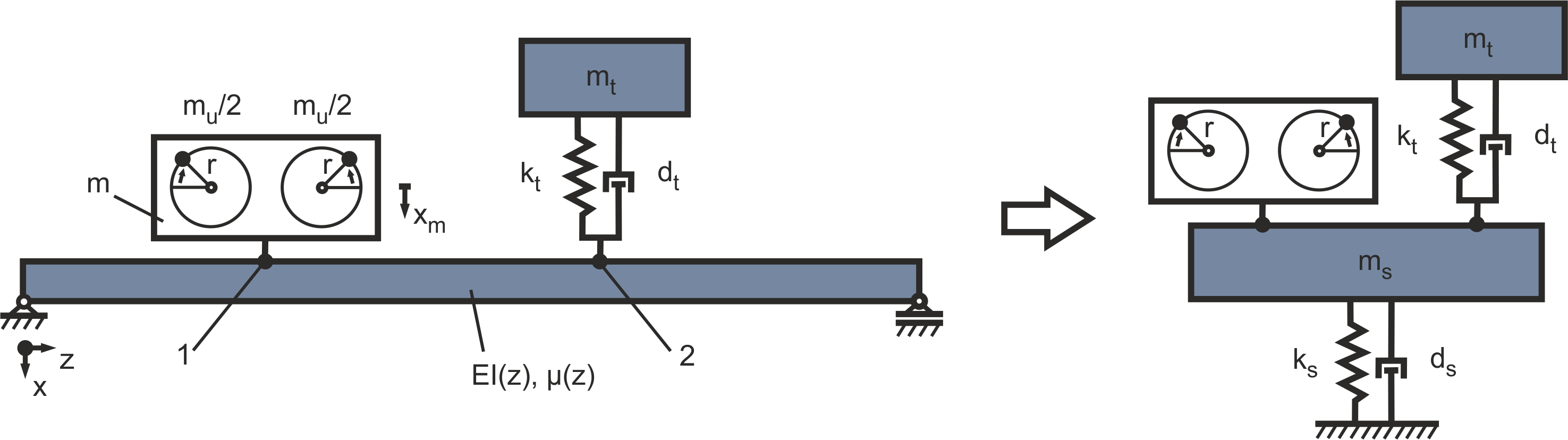
Figure 14: Rigid bearing with absorber
For an effective reduction effect, the absorber must be tuned to the natural frequency of the structure. The appropriate selection of the parameters mt, kt is therefore crucial. However, the tuning of the damping also influences the properties of the absorber. As analytical optimisation of the parameters is complicated, the parameters are estimated and the quality of the solution is evaluated and adjusted using the graphical representation of the transmission. The stiffness is to be calculated taking into account the dominant resonant frequency of the rigidly coupled motor f1 = 14.411 Hz. The stiffness can be estimated from  . The degree of damping D should be between 5% and 20%. By this the damping dt can be determined by
 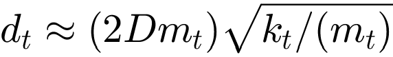 . When parameterising vibration dampers, it should be noted that the parameters mt, kt and dt are mutually dependent. An iterative approach is therefore recommended to optimise the parameters. The resulting curve provides information about the quality of the parameters. Figure 15 a – c shows the influence of the parameters on the curve. One parameter was varied in each case to show the influence on the curve, while the other two parameters were adjusted to achieve the best possible curve. [3]
|
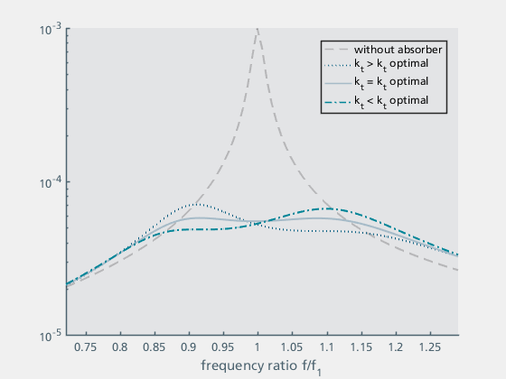
Figure 15a: Variation of kt |
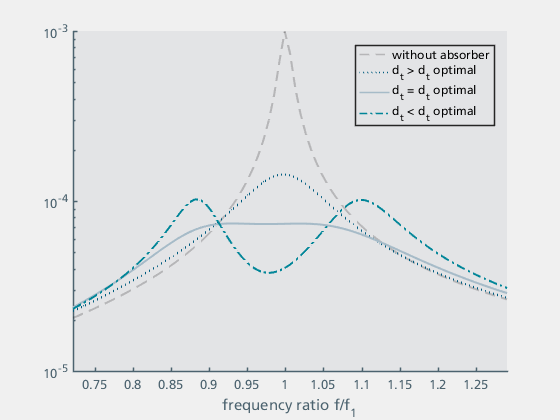
Figure 15b: Variation of dt |
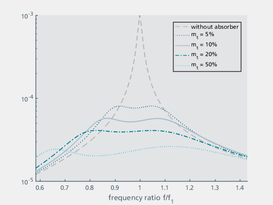
Figure 15c: Variation of mt |
| Figure 15a shows the influence of the stiffness kt. The case without absorber is also shown for comparison. The stiffness kt and the mass mt determine the absorber frequency ft. The curves of the structure with absorber shows two hills that are the same height at the optimum frequency. The hills are below and above the natural frequency of the structure. If the absorber frequency is too low (or the stiffness is too low), the upper hill is too high, if the absorber frequency is too high (or the stiffness is too high), the lower hill is too high. | Figure 15b shows the curves for different absorber dampings dt. If the damping is too low, both hills are too high, if the damping is too high, only one hill remains in the centre, which is also too high. | Figure 15c shows the curves for different ratios of the absorber mass mt to the supporting structure mass (mges). It can be seen that the damping effect increases with increasing absorber mass and at the same time the curve becomes wider. In practice, higher absorber masses are associated with higher manufacturing and assembly costs for the vibration absorber as well as additional static loads. For this reason, an absorber mass of between 5% and 20% is usually selected as a compromise. |
Implementation in Simulink
To simulate the absorber, the simulink model from Figure 4 was extended to include an absorber mass and a spring-damper element (see Figure 16).

Figure 16: Simulink model of the rigidly mounted motor with absorber
An absorber mass mt of 100 kg was assumed. This corresponds to a mass ratio mt/mges of approx. 12 %. The stiffness kt was estimated in a first step with  . This results in a value of 8.1984e+05 N/m. The values 905.45 kg*s and 3621.8 kg*s were used as the damping constant of the absorber. This corresponds to a damping factor of 5% and 20% respectively. In addition, the simulation was carried out with an iteratively optimised value for kt_opti = 688660 N/m. A damping factor of 20% was used here, which corresponds to a damping constant of 3319.4 kg*s. Figure 17 compares the various simulation results with the results of the rigidly mounted motor without absorber in the frequency range.
▾ Show source code
% Display simulation data in time domain

simout_label = {'d_t = 5%','d_t = 20%','Iteratively optimised'};

[FREQ_0,AMPL_0,PHAS_0]=ma_frequency_response(time_0, F_0, x_0,{0,50},'window',true);
h = figure();
ma_graphics.semilogy(FREQ_0,AMPL_0);
hold on;
for ind = 1:3
    [FREQ_t(:,ind),AMPL_t(:,ind),PHAS_t(:,ind)]=ma_frequency_response(time_t(:,ind), F_t(:,ind), x_t(:,ind),{0,50},'window',true);
     ma_graphics.semilogy(FREQ_t(:,ind),AMPL_t(:,ind));
     grid on
     xlabel('Frequency in Hz')
     ylabel('Amplitude in m/N')
end
legend('Stiff coupling',simout_label{:},'Location','best')
xlim([5 50])
a=rectangle('Position',[f_u_min,1e-6,f_u_max-f_u_min,1.9e-4],'FaceColor',[0 .5 .5 0.2],'EdgeColor','b', 'LineWidth',1);
% push rectangle (last plot) to the back
ah = get(gca,'Children');
set(gca,'Children',[ah(2:end)',ah(1)]);
text(14,1.5e-6,'Operation range')
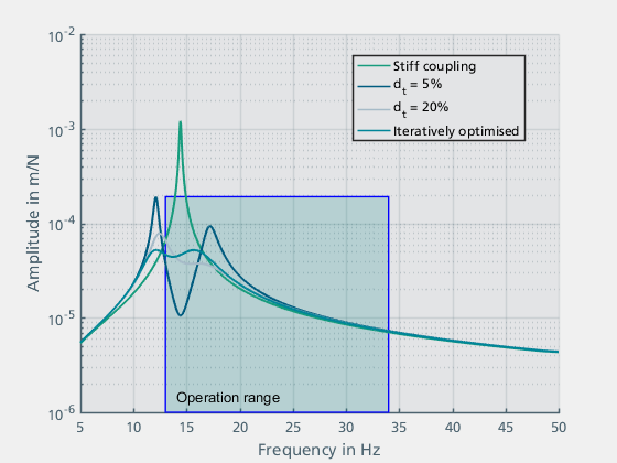
Figure 17: Results of the reduction effect by an absorber with a damping factor of 5% and 20% as well as an iteratively optimized value for kt
For the lightly damped system, the resonance is damped, creating two neighbouring resonances. These result from the additional degree of freedom introduced into the system. With the higher damping, the amplitude of the neighbouring resonances is smaller, whereby the efficiency of the reduction effect also decreases. The curve for the iteratively optimised parameter kt is almost linear. As the first resonance frequency of the absorber is outside the operating range, it would also be possible in this case to optimise the parameters kt and dt so that the amplitude of the second resonance frequency is as small as possible.
Comparison with the analytical solution
To compare the simulation results with the analytical solution, the system matrices of the iteratively optimised values are derived using the ma_mosys class and compared with the simulation results.
▾ Show source code
% Define the mass matrix of the system, where the first entry defines the mass annotation
jData = [1 m_s+m_m;
         2 m_t];

% Define arrangement of the masses and the spring and damper values of the respective connections
kData = [1 inf k_s d_s;
         1 2   k_t_opti d_t_opti];

% Force application points of the system
originFvalue = 1;

% Output velocity masses of the system
outputPvalue = 1;

system = ma_mosys(jData,kData,'originF',originFvalue,'outputP',outputPvalue);

% Create the state-space model
system.getSS;

% Use the matlab built-in function eig to calculate the eigen values
eigenValues = eig(system.SS);
eigenFrq_t = unique(abs(eigenValues))/(2*pi);

freq_analytic=0:0.1:50;
[mag_analytic, phase_analytic]=bode(system.SS,freq_analytic*2*pi);
mag_analytic = reshape(mag_analytic,1,length(freq_analytic));

h = figure();
ma_graphics.semilogy(FREQ_t(:,3),AMPL_t(:,3));
hold on;
ma_graphics.semilogy(freq_analytic,mag_analytic);
hold off;
grid on
xlabel('Frequency in Hz')
ylabel('Amplitude in m/N')
legend('Simulink','Analytic')
xlim([5 50])
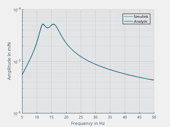
Figure 18: Comparison of the Simulink model with the analytical solution
Figure 18 shows that the results of the simulation and the solution of the analytical model match. The calculated natural frequencies 11.985 Hz and 15.88 Hz also agree with the observed resonance frequencies.
Combination of vibration isolation with an absorber
In the previous sections, vibration isolation and the use of a vibration absorber were considered separately. In order to achieve optimum vibration reduction, both structural-dynamic measures are combined in the following (Figure 19).
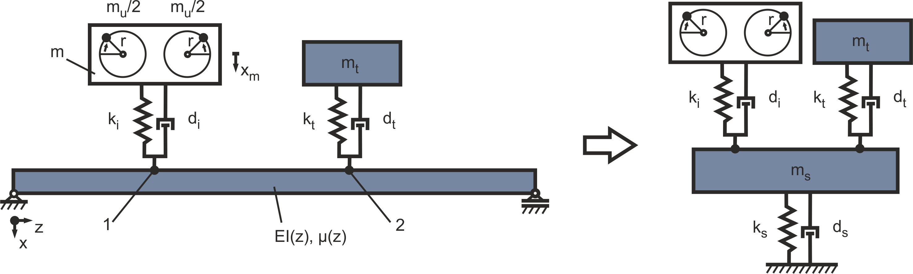
Figure 19: Elastic mounting with vibration absorber
Firstly, the spring and damping values of the absorber must be adapted to the resonant frequency of the elastically mounted motor (see section: Passive isolation using elastic mounts). The mass of the absorber is again assumed to be mt = 100 kg. As only the mass of the motor is taken into account in this case, this corresponds to a mass ratio of 17%. Based on the resonant frequency of 32.541 Hz prevailing in the operating range, the value for kt is initially estimated to be 4.1803e+06 N/m with 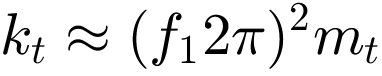 . This results in a value of 2044.6 kg*s for the damping constant dt at a damping factor of 5% and a value of 8178.3 kg*s at 20% damping. Here too, the values for kt and dt were then iteratively optimised and determined as 2090200 N/m and 7228.8 kg*s.
Implementation in Simulink
Figure 20 shows the Simulink model of the elastically mounted motor with vibration absorber.

Figure 20: Simulink model of the elastically mounted motor with vibration absorber
Figure 21 shows the simulation results with a damping factor of 5% and 20% as well as the result of the iteratively optimised parameter values.
▾ Show source code
simout_label = {'d_t_i = 5%','d_t_i = 20%','Iteratively optimised'};
h = figure();
ma_graphics.semilogy(FREQ_0,AMPL_0);
hold on;
for ind = 1:3
[FREQ_t_i(:,ind),AMPL_t_i(:,ind),PHAS_t_i(:,ind)]=ma_frequency_response(time_t_i(:,ind), F_t_i(:,ind), x_t_i(:,ind),{0,50},'window',true);
    ma_graphics.semilogy(FREQ_t_i(:,ind),AMPL_t_i(:,ind));
end
legend('Stiff coupling',simout_label{:},'Location','best')
xlim([5 50])
rectangle('Position',[f_u_min,1e-6,f_u_max-f_u_min,1.9e-4],'FaceColor',[0 .5 .5 0.2],'EdgeColor','b', 'LineWidth',1);
% push rectangle (last plot) to the back
hc = get(gca,'Children');
set(gca,'Children',[hc(2:end)',hc(1)]);
text(14,1.5e-6,'Operation range')
grid on;
xlabel('Frequency in Hz')
ylabel('Amplitude in m/N')
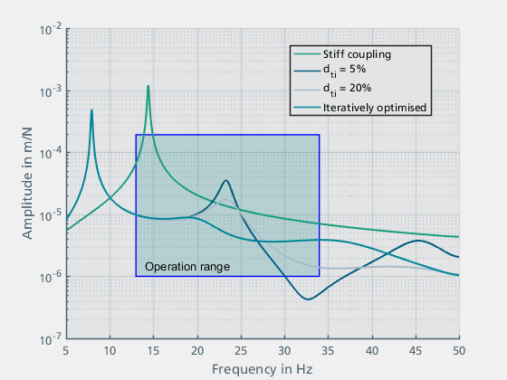
Figure 21: Simulation results of the elastically mounted motor with vibration absorber
Concluding considerations
This tutorial showed how unwanted vibrations can be reduced by structural dynamic measures. Using the model of an internal combustion engine in a ship, the influence of an elastic mounting and a vibration absorber was discussed and it was shown how the dynamic behaviour can be simulated and evaluated using elements of the ma_Toolbox. Figure 22 compares the simulation results of the various measures. Elastic mounting of the motor isolates the excitation. This significantly reduces the vibrations introduced into the basic structure. However, a new resonance occurs in the higher frequency range, the amplitude of which is greater in this range than with the rigid mounting. By using a vibration absorber, it is possible to significantly reduce the amplitude in the range of the natural frequency of the basic structure. The influence of the stiffness and damping factors of the absorber was discussed in this context. A low damping factor results in new resonant frequencies, while a higher damping factor significantly reduces the effectiveness of the absorber. The combination of both measures leads to the best results over the entire operating range. In this case, the vibration absorber is designed for the resonance frequency resulting from the elastic mounting.
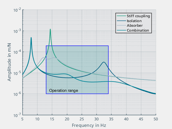
Figure 22: Comparison of the reduction effects of the various methods
Literature
[1] Grote, K.-H.; Feldhusen, J. (Hg.) (2014): DUBBEL – Taschenbuch für den Maschinenbau, DOI: https://doi.org/10.1007/978-3-642-38891-0
[2] Böge, A.; Böge, W. (Hg.) (2021): Handbuch Maschinenbau – Grundlagen und Anwendungen der Maschinenbau-Technik, DOI: https://doi.org/10.1007/978-3-658-30273-3
[3] Weber, B. (2012): Tragwerksdynamik, DOI: https://doi.org/10.3929/ethz-a-007362062
[4] Preumont, A. (2011): Vibration Control of Active Structures – An Introduction, DOI: https://doi.org/10.1007/978-94-007-2033-6For