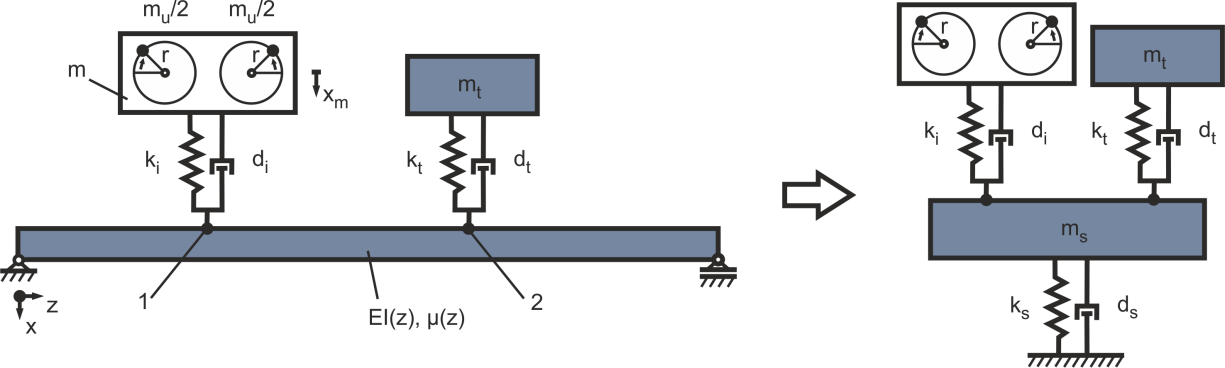
Figure 16: Simplification of the structure with an elastic mounting of the excitation and a tuned mass-damper
Implementation in Simulink®:
By this means a Simulink® simulation model due to the previous evaluated parameters for the isolation is set up. For the mass of the tuned mass-damper mi = 100 kg is used. The stiffness is set up with regards to the governing resonance in the operating range of the machine at f1 = 32.3 Hz By this means a stiffness of kt=(f1 2π)^2 * mt= 4.1187e6 N/m is used. The resulting Simulink® block-diagram of the damped harmonic oscillator with combination of the isolation and the tuned mass-damper is pictured in Figure 15.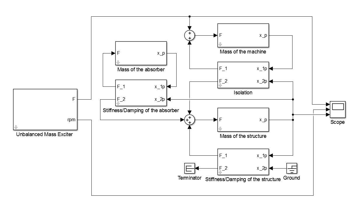
Result:
For time-domain simulations a Simulink® model is implemented as seen in Figure 17. For the parametrization the properties listed in Table 1 are used.
[FREQ,AMPL,PHAS]=ma_frequency_response(ScopeData.time, ScopeData.signals(1).values,
ScopeData.signals(3).values,{0,50});
[FREQ_Damping,AMPL_Damping,PHAS_Damping]=ma_frequency_response(ScopeData_Damping.time,
ScopeData_Damping.signals(1).values, ScopeData_Damping.signals(3).values,{0,50});
[FREQ_Isolation,AMPL_Isolation,PHAS_Isolation]=ma_frequency_response(ScopeData_Isolation.time, ScopeData_Isolation.signals(1).values, ScopeData_Isolation.signals(3).values,{0,50});
[FREQ_Combination,AMPL_Combination,PHAS_Combination]=ma_frequency_response(ScopeData_Combination.time, ScopeData_Combination.signals(1).values, ScopeData_Combination.signals(3).values,{0,50});
figure
semilogy(FREQ,AMPL,’k’,’LineWidth’,2); hold on;
semilogy(FREQ_Damping,AMPL_Damping,’b’,’LineWidth’,2);
semilogy(FREQ_Isolation,AMPL_Isolation,’r’,’LineWidth’,2);
semilogy(FREQ_Combination,AMPL_Combination,’g’,’LineWidth’,2);
hold off;
grid on
xlabel(‘Frequency in Hz’)
ylabel(‘Amplitude in m/N’)
legend(‘Stiff coupling’,’Mass-damper (\xi=5%)’,’Isolation’,’Combination’,’Location’,’SouthWest’)
xlim([5 50])
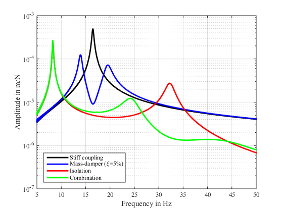 Figure 18: Frequency domain results in with a mass-damper, isolation and the combination of both |
In Figure 18 the different measures are compared in the frequency domain. The tuned mass-damper results in an efficient reduction of the combined resonance of the structure and the machine. Nevertheless still either neighboring double-peaks remain or the effect is reduced. The isolation reduces the resonance better and shifts the frequency higher and still to a higher amplitude, than the stiff coupling. This resonance can reduced due to the use of an additional mass-damper tuned to the remaining resonance. This way the combination shows practical no disadvantage in regard of an increasing peak over the base level of the stiff coupling.