It is possible to reduce vibrations by applying additional structural-dynamic measures like damped mass-spring-dampers. Here the reduction of the vibrational level in the domain of a structural resonance is possible. The introduced example in Figure 1 (from example Bearing Structure) can be simplified to the setup in Figure 12. Here both the force excitation in position 1 and the position of the tuned mass-damper 2 are considered collocated..
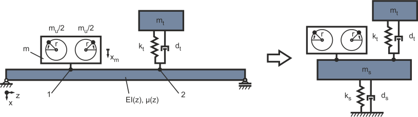
Figure 12: Simplification of the structure with an elastic mounting of the excitation
Implementation in Simulink®:
For a sufficient damping effect an essential mass is necessary. By a rule of thumb a damping mass of 5 % to 20 % of the effective vibrating mass of the base structure is considered [5]. For the regarded mass-damper a mass of mt = 100 kg is considered. The stiffness is set up with regards to the governing resonance of the coupled machine with the structure at f1 = 16.5 Hz. By this means a stiffness of kt=(f1 2π)^2 * mt = 1.0748e06 N/m is used. The resulting Simulink® block-diagram of the damped harmonic oscillator with the tuned mass-damper is pictured in Figure 13.
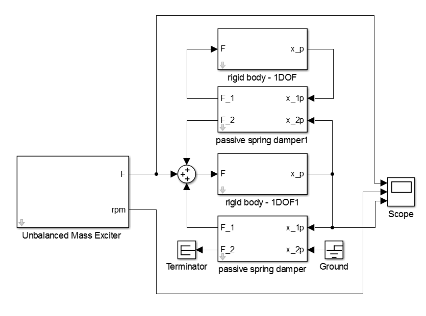
For time-domain simulations a Simulink® model is implemented as seen in Figure 13. For the parametrization the properties listed in Table 1 are used. For the damping of the mass-damper an amount of 1000 kg*s and 4000 kg*s is used representing a damping ratio of 5% and 20%.
Result:
The frequency domain is evaluated by the use of the ma_frequency_response function:
[FREQ,AMPL,PHAS]=ma_frequency_response(ScopeData.time, ScopeData.signals(1).values,
ScopeData.signals(3).values,{0,50});
[FREQ_Damping,AMPL_Damping,PHAS_Damping]=ma_frequency_response(ScopeData_Damping.time,
ScopeData_Damping.signals(1).values, ScopeData_Damping.signals(3).values,{0,50});
figure
semilogy(FREQ,AMPL,’k’,’LineWidth’,2); hold on;
semilogy(FREQ_Damping,AMPL_Damping,’r’,’LineWidth’,2);
hold off;
grid on
xlabel(‘Frequency in Hz’)
ylabel(‘Amplitude in m/N’)
legend(‘Stiff coupling’,’Mass-damper (\xi50%)’,’Location’,’SouthWest’)
xlim([5 50])
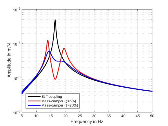
In Figure 14 the results of the simulation with a damping ratio of 5% and 20% can be seen in the frequency domain. For the lightly damped system the resonance of the structure is damped with additionally occurring two neighboring peaks. This result of the additional degree of freedom introduced to the system by the tuned mass-damper. For the higher damping the resulting double peaks are smaller. This advantage also has the drawback of a lower efficiency regarding the damping effect. For an analytical comparison the system matrices can be derived using the function ma_MOSys from the structure and vibration package :
% jData definition of sys1
jData = [1 882.6;
2 100];
% kData definition of sys1
kData = [1 inf 9470328 2000;
1 2 1.0748e6 1000];
% originF definition
originFvalue = 1;
% outputP definition
outputPvalue = 1;
Sys1 = ma_MOSys(jData,kData,’originF’,originFvalue,’outputP’,outputPvalue);
By this means the system is transferred to a state-space system and the eigenvalues are calculated:
ss = ma_MOSysGetSS(Sys1);
eig(ss)
As result the eigenfrequencies 19.47 Hz and 13.96 Hz are calculated which match the Simulink® simulation. For a match of the amplitudes the frequency response functions are compared:
freq_analytic=1:0.1:50;
[mag_analytic, phase_analytic]=bode(ss,freq*2*pi);
mag_analytic=reshape(mag_analytic,1,length(freq));
[FREQ_Damping,AMPL_Damping,PHAS_Damping]=ma_frequency_response(ScopeData_Damping.time,
ScopeData_Damping.signals(1).values, ScopeData_Damping.signals(3).values,{0,50});
figure
semilogy(FREQ_Damping,AMPL_Damping,’k’,’LineWidth’,2); hold on;
semilogy(freq_analytic,mag_analytic,’r’,’LineWidth’,2);
hold off;
grid on
xlabel(‘Frequency in Hz’)
ylabel(‘Amplitude in m/N’)
legend(‘Simulink’,’analytic’,’Location’,’SouthWest’)
xlim([5 50])
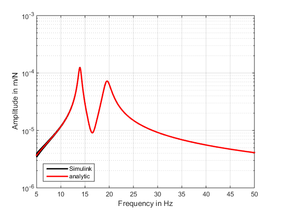 Figure 15: Match of the Simulink® model with the analytic solution |
As one can clearly see in Figure 15, the analytic solution matches the Simulink® simulation quite good.